For Chinese users, the answer to this question can be found in section 9.5 of white book v2 (http://newshxmt.ihep.ac.cn/images/proposal/whitebook_v2.pdf). For users in other countries, the translation of that section is provided as below:

The Insight has three slat-collimated instruments: the Low Energy X-ray Instrument (LE), the Medium Energy X-ray Instrument (ME), and the High Energy X-ray Instrument (HE).

The energy bands are: LE：1-11 keV，ME: 10-35 keV, HE：28-250 keV

Warning: Simulation should be made within the energy bands provided above.

The fakeit tool in XSPEC of HEASOFT is used for the simulation. The response and background files are packaged in 'user_spec_2018_2019.zip', the download website for which is http://proposal.ihep.ac.cn/soft/soft.jspx. The background spectra are in the 'bkg_fits' directory of each instrument; the response files are in the 'rsp' directory of each instrument; the example scripts are in the 'example' directory.

We now give an example on how to simulate an observed spectrum (background included) at a given length of exposure. To make the example simple, we assume there is no other source inside the FOV (field of view) of the target source. We further assume the spectrum model is a single power-law without interstellar absorption (the 'powerlaw' model in XSPEC with PhoIndex=1.7 and norm=10 photons keV-1 cm-2 s-1@1 keV).

Step 1: run XSPEC and establish the spectral model:

Run XSPEC and type 'mo pow' to establish the spectral model. Then type the value of each parameter according to the prompt. Finally type 'save mo inputmodel.xcm' to save the spectral model in a file with name of 'inputmodel.xcm'. Above process is shown in figure 1 below. Users can choose not to save the 'inputmodel.xcm' file, but to run fakeit next. The advantage of saving the 'inputmodel.xcm' is that users need not to establish the spectral model every time when using it, but to type '@inputmodel.xcm' in XSPEC to load the spectral model easily. 

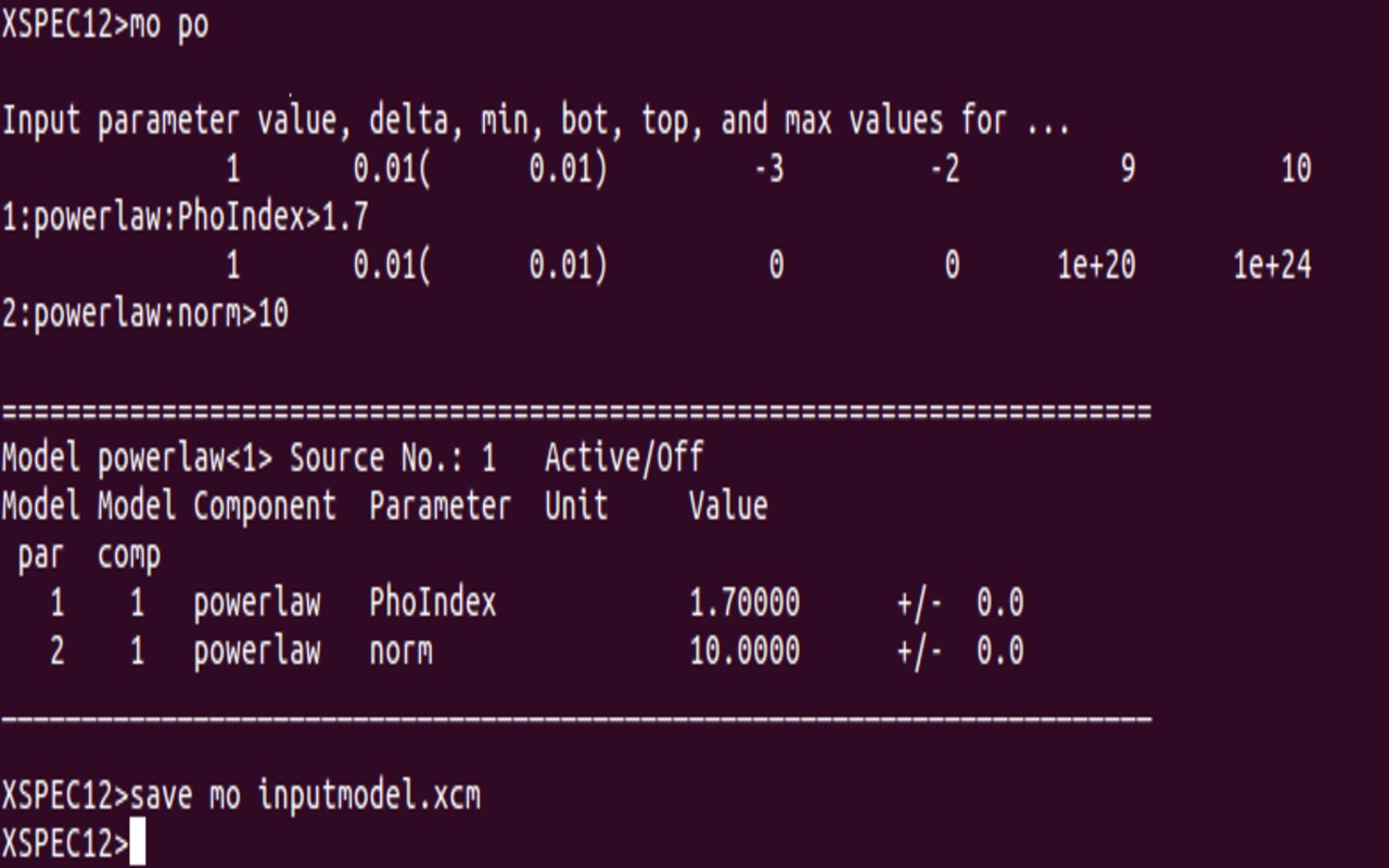
Figure 1 the process of establishing the spectral model of the target source.

Since LE, ME, HE are slat-collimated instruments with large FOV (field of view), there might be other sources in the FOV of the target source. For how to find the nearby bright sources, please refer to the FAQ item 'How do I estimated the effects of the bright sources nearby?'. But it should be noticed that the intensity of those sources might be variable. If there are other bright sources in the FOV of the target source, they should be considered when users are establishing the above 'inputmodel.xcm' file. This issue is discussed in detail in the final part of this section.

Step 2: use 'fakeit' to simulate the spectrum

Taking ME for example, if we want to simulate a spectrum with 10000 s net exposure, after step 1, we may type the sentence below in XSPEC:

fakeit ME_bg.fits & MEPI_20181207.rmf & MEPI_20181207_tot.arf & y & & ME_tot.fak & 10000, 1, 10000;

In that sentence, ME_bg.fits is the background spectrum, and MEPI_20181207.rmf and MEPI_20181207_tot.arf are the RMF and the ARF files for ME respectively (the website for downloading them is already provided in the beginning of this section). 'y' means counting statistics is used in creating fake data (the corresponding prompt is'Use counting statistics in creating fake data？'). Usually we choose 'y' for this prompt, because there is counting statistics in real observations.

These two warnings appeared should be ignored:

Warning: RMF INSTRUMENT keyword is not consistent with spectrum

Warning: RMF CHANTYPE keyword (PI) is not consistent with that from spectrum (PHA)

After running the above fakeit sentence, two simulated spectra are obtained. One is the total observed spectrum 'ME_tot.fak' (source and background are both included). The other is the estimated background spectrum 'ME_tot_bkg.fak' which is used to estimate the background in the total spectrum 'ME_tot.fak'. (Different from 'ME_tot.fak', the statistic error of 'ME_tot_bkg.fak' is relatively small, because it has used the data with long exposure in the database). Those two spectra are enough for users to do spectral analysis. They are the input total spectrum and the background spectrum when using XSPEC to fit the spectrum. It should be noticed that if the counts in each channel is not large enough for the need of XSPEC, users should rebin the spectra before fitting in XSPEC. In addition, it should be noticed that the systematic error of the estimated background spectrum 'ME_tot_bkg.fak' is not considered in above example. Actually, it is small. The systematic errors of the estimated background spectra'HE_tot_bkg.fak', 'ME_tot_bkg.fak', and'LE_tot_bkg.fak' are 1%, 3% and 2% respectively. Users can choose whether to consider them or not according to the case.

Warning!!! when fitting the spectrum, please use the correct energy band, which is listed in the beginning of this section!!!

Sometimes it is necessary to rebin the spectrum when using XSPEC to fit the spectrum. Users can rebin the spectrum by himself/herself. The GRPPHA software can also be used to rebin the spectrum.

Above we run fakeit by using a sentence containing parameters. Users can also type fakeit ME_bg.fits in XSPEC and then press 'Enter', and then type each parameter according to the prompt.

Above we use ME to illustrate the simulation process. The simulation of HE and LE is similar to ME except that their response and background files are different. It should be emphasized that HE has 17 detectors to observe the source, and their spectra are simulated separately. When then 17 spectra have been simulated, users can fit them together in XSPEC. (HE has 18 detectors in total with IDs 0-17. The detector with ID 16 has its FOV (field of view) covered, thus it does not observe the source). For ME and LE, the simulated spectrum is the total spectrum of the instrument. We provide example scripts for the simulation of HE, ME and LE, which are in the directory 'example' in 'user_spec_2018_2019.zip' mentioned in the beginning of this section. Users can choose whether to use them or not. The scripts are written in TCL language. They can be invoked by using '@' in XSPEC. For example:

XSPEC12>@HE.tcl

or invoked in the terminal directly:

xspec - HE.tcl

Similarly, these two Warnings appeared can be ignored:

Warning: RMF INSTRUMENT keyword is not consistent with spectrum

Warning: RMF CHANTYPE keyword (PI) is not consistent with that from spectrum (PHA)

Below, we will illustrate how to establish the spectral model file in the case where there are other bright sources in the FOV:

We discuss the situation that the target source is on axis, while there are other bright off axis sources which are also in the FOV. Since Insight is a slat-collimated instrument, photons from those off axis sources will contribute to the total counts. Below we call those off axis sources 'polluting sources'. Polluting sources can be divided into two types: one is the newly bursting source whose position is unknown; the other is the source already known. We only consider the second case.

For the second case, the positions of the polluting sources are known. The attitude of the instrument will be adjusted to avoid those sources as much as possible. However, sometimes they can still not be avoided. Below we will give an example where there is only one polluting source (the method of dealing with multiply polluting sources is similar):

We call the spectral model of the target source model1, and that of the polluting source model2. Then, in the case where there is no polluting source, the 'inputmodel.xcm' file mentioned above gives model1. If the polluting source is bright enough that must be considered, the spectral model in the 'inputmodel.xcm' file should be set to 'model1 + constant * model2', where constant is also a model in XSPEC, which is a constant whose value can be set by users. constant may include (but not limit to) the product of two factors: one is the variability of the intensity of the polluting source; the other is denoted as f, which is the ratio of the number of photons arriving the detector when the polluting source is off axis to when it is on axis. The range of f is 0 to 1.

The value of f is determined by two factors. One is the angular distance between the target source and the polluting source. This factor is known. The other is the attitude of the instrument, which is related to the relative position of the Sun to the instrument, hence related to time when the observation will be carried out. That cannot be totally determined. However, we can give the range of f in figure 2. Users can give an optimistic and a pessimistic estimation according to it. f is different for HE, ME and LE.­­

Figure 2 The x axis is the angular distance between the target source and the polluting source. The y axis is the value of f, with * denoting the minimal possible value and diamond denoting the maximal value. The top, middle and bottom are for HE, ME and LE, respectively.

Any question please contact: jjin@ihep.ac.cn